Machine Learning & Food Classification
Between April and October of this year I completed the Data Science Intensive course administered by Springboard, and my capstone project involved attempting to train a machine learning algorithm to correctly classify pictures of food dishes.
The purpose of this post is to try and explain some of the underlying models and the results in a relatively non-technical way.
1. Project motivation
2. The Problem and Definition of Success
3. General Approach and Data
4. Traditional Machine Learning: Algorithms
5. Traditional Machine Learning: Features
6. Deep Learning & Neural Networks
7. Results
8. Visualizing a Network
9. Summary
1. Motivation
Perhaps the first question might be, why do you care about food classification?
The truth is that food classification is just a means to an end; I wanted to learn more about computer vision techniques, but in order to do this I needed to work on a tangible problem. I chose food classification because it let me apply what I was learning to one of my favourite pastimes: food and cooking.
Having said that, this is not just a toy problem. There are many potential applications for a successful food classification algorithm. For example, when people are searching for recipes it is now quite common to turn to websites and apps to find food-related content. One very simple application could be for recipe search and retrieval using a picture of a dish, such as something you tried while traveling but whose name you have now forgotten.
As another example, there are already researchers working on food classification tied-in with food calorie data in order to help people easily keep a daily food diary and calorie count, perhaps enabling them to better control their food intake and stick to a diet.
However, that is all that I will say about applications, as the real aim is to develop a better understanding of the techniques behind machine learning, in particular when applied to image classification.
2. The Problem and Definition of Success
I have already hinted at the problem, however it will be useful to make this more formal.
Specifically, we are faced with a classification problem. Given a set of images of different types of food, we wish to find an algorithm that can be 'shown' an image and correctly categorize it into one of the pre-defined categories.
There are a couple of important points to note about this type of problem:
- The categories are pre-defined and fixed; the algorithm is only going to be capable of categorizing an image into a 'known' category or class. It will not be able to identify new food categories on the fly.
- We limit the problem to identifying single categories for each image, or in other words the algorithm must decide whether an image is of Pizza or Steak etc. There are computer vision techniques for identifying multiple objects in a single image, however these are beyond the scope of this project.
Definition of Success
Something else that should be defined in advance is the definition of success: how should different algorithms' performance be evaluated?
One very simple measure could be the classification rate, that is the total number of correct predictions divided by the total number of predictions made.
Whilst this does measure predictive success, this metric does not quite capture all of the subtleties of classification. Instead we will use a metric called the F1-score, illustrated using the following simple example.
Consider a reduced version of the problem looking at categorising images into Pizza or Not Pizza. Typically, when 'shown' an image, an algorithm outputs probabilities for each outcome rather than a definitive answer.
For example, given a new image, the algorithm may output:
- Pizza: Probability = 0.6
- Not Pizza: Probability = 0.4
In order to translate these probabilities into a prediction, we must set a probability cut-off, or threshold, for Pizza, whereby any score above that threshold is a Pizza prediction, and any score below becomes Not Pizza. In this example, if we set the threshold at 0.5, then the image would be classified as Pizza (as 0.6 > 0.5).
Now imagine that we show 100 images to the classification algorithm, and we summarize the resulting predictions in a table (commonly called the confusion matrix).
| Predicted Category | |||
|---|---|---|---|
| Pizza | Not Pizza |
||
| Actual Category | Pizza | True Positive | False Negative |
| Not Pizza |
False Positive | True Negative | |
The rows represent the True Category of the images, and the columns represent the Predicted Category. These outcomes can be summarized in the following way:
- True Positives: Top-left corner; images of Pizza correctly classified as Pizza.
- False Negatives: Top-right corner; images of Pizza incorrectly classified as Not Pizza.
- False Positives: Bottom-left corner; images that are Not Pizza incorrectly classified as being Pizza.
- True Negatives: Bottom-right corner; images that are Not Pizza correctly classified as being Not Pizza.
We can now define two metrics.
One way to think about Precision is that it measures, out of all images predicted to be Pizza, what proportion actually are Pizza. In some senses this tells us how noisy our Pizza predictions are, or how much the algorithm confuses other types of food with Pizza.
Similarly Recall asks, out of all true Pizza images, what proportion were correctly identified as being Pizza. This is a measure of how good the algorithm is at correctly identifying pizza images and placing them in the correct category.
It turns out that by varying the probability classification threshold mentioned above, you can tune the Precision and Recall scores for the classification algorithm.
Suppose, for example, that you want to maximize Precision; in practice this means minimizing the False Positives or, in other words, requiring the algorithm to output Pizza only when it is very confident that the image is of Pizza. In order to achieve this, you can increase the threshold probability thus ensuring that Pizza predictions are only made when the probability is high for Pizza.
Similarly, by decreasing the probability threshold, you can get the algorithm to classify images as Pizza, even when its confidence is low, thus minimising the False Negatives and resulting in higher Recall. This might be important in other applications, for example when using Machine Learning to detect cancerous cells, where the cost of False Negatives is higher than the cost of False Positives.
Although one could use either Precision or Recall as a way of measuring algorithm performance, ultimately both are important. Thus we define the F1 score to be:
This particular definition gives equal weighting to both Precision and Recall, however it is possible to adapt the formula to give more weighting to one or the other. F1 is measured on a scale from 0 to 1, with 1 being the best possible score.
3. General Approach and Data
We now have a definition of the problem:
Find an algorithm that can take an image as input, and output a prediction for the category of food contained in the image
as well as a measure of success, the F1 score.
One way to approach this problem could be to try and manually create a list of rules in order to distinguish between different kinds of food. For example, if you wanted to distinguish between pictures of apples and bananas, you could attempt to construct rules that look at shape, size, colour etc.
However, as we know from experience, apples can come in a wide variety of colours, bananas in very different shapes etc., so coming up with an exhaustive set of rules could become overwhelming quite quickly. The problem is even worse when we look at complex food dishes rather than single ingredients.
For this reason, rather than using this rule-based approach, we turn to a field called Machine Learning.
Machine Learning
Arthur Samuel, a pioneer of the field, defined Machine Learning as a:
"Field of study that gives computers the ability to learn without being explicitly programmed”
At the heart of Machine Learning are algorithms that are able to build an internal representation or model of some data, without us having to explicitly program the model ourselves.
Such algorithms can then use this internal model in order to make predictions about new data points.
We will specifically focus on a particular type of machine learning called Supervised Learning.
Supervised Learning
In supervised learning, we start with a relevant set of data that has already been classified into the different categories of interest. In the specific case of this project, this means that someone has looked at every single image in the dataset and manually attached a label to each image.
This labeled data is then used for a period of training in which we "show" each image to the algorithm along with the correct answer and the algorithm attempts to use this information to build a generalized model that can accurately map inputs (the training image data) to outputs (predictions of food categories).
As will be seen in later sections the specifics of the internal model vary greatly between algorithms. Furthermore, when we "show" images to the algorithm during training, some algorithms use the entire image, pixel by pixel, whereas others use other types of data extracted from the each image.
The key to supervised learning is in having data where you know the categories, or answers, in advance, and using these answers to teach the algorithm how to make predictions about new data.
The Dataset
For this particular problem we need a set of training data that consists of a large number of pre-categorized pictures of different types of food. The dataset that we will work with comes from the ETH Zurich Computer Vision Laboratory, and is called the Food 101 Dataset.
This dataset consists of 101 different food categories, with 1,000 images per category, for a total of 101,000 images. However the total dataset is too large for practical experimentation on a laptop, and so in order to reduce the complexity, we will focus on 12 categories out of the whole list:
| Pork Chop | Lasagna | French Toast |
| Guacamole | Apple Pie |
Cheesecake |
| Hamburger | Fried Rice |
Carrot Cake |
| Chocolate Cake |
Steak | Pizza |
The images in the Food-101 dataset are of mixed quality. Some are very clear, well-lit and framed on the food item in question. Others, however, are more noisy, poorly lit, contain irrelevant items and, in some cases, are even mislabeled. Some examples of both high and low-quality pictures are shown below:
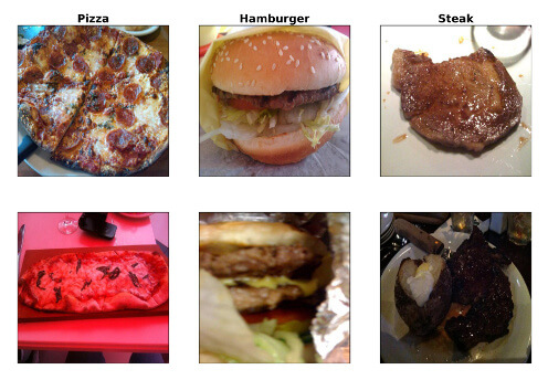
In some respects this 'noise' in the data makes the problem harder, as the algorithm will need to differentiate between types of food that are not so easy to distinguish, as well as correctly identify food categories from images that vary significantly in terms of lighting and image quality.
At the same time, this also means that if we are able to train a classifier to a sufficient level of accuracy, then we might expect its predictions to be more robust when used on real-world, equally-noisy data.
Using Data
Before moving on to looking at different types of algorithms, it is important to note the general methodology for using data in Supervised Machine Learning problems.
As mentioned, we are starting with a set of 12,000 images, equally divided into 12 categories, however not all of the images will be used during training.
Instead, before doing anything else, we will split the dataset into two random subsets for training and testing purposes. The training data is what we will show the algorithm along with the relevant answers during the training phase. The testing data is used exclusively for evaluating how well a given algorithm works in practice.
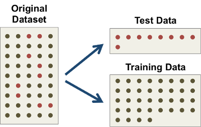
This is a general pattern for data usage that applies to any supervised approach. It is absolutely key that the test data is not used at all during algorithm training, otherwise any predictions made on that data could be considered 'cheating', and ultimately we will not know how well the algorithm could perform in the real world on previously unseen data.
In an ideal world, when working on a supervised learning problem, one would be able to ring-fence somewhere around 15 to 20% of the data for testing purposes. In reality, the exact strategy and percentage used will depend on the nature of the problem as well as the actual available data.
4. Traditional Machine Learning: Algorithms
We start by exploring techniques from a traditional machine learning approach in which two key choices must be made:
- The type of algorithm to train, and
- The type of data to use during training
There are a wide variety of machine learning algorithms that could be used, and we will briefly explore three examples below.
k-Nearest Neighbours
k-Nearest Neighbours (kNN) is one of the simplest supervised learning algorithms, and has the benefit of being very easy to use, visualize and understand.
The basic methodology for making a prediction is:
- Find the k 'closest' neighbouring images within the training dataset
- Look at the category for each of these neighbours
- Combine the category for each neighbour into an overall prediction
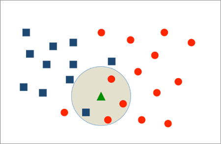
In the example below there are two categories, Red and Blue. Given a new data point (the green triangle) we look at the 4 nearest neighbours of which three are Red and only one is Blue, and so we would classify the new point as being Red.
Some specific parameters we can define for the algorithm are:
- How many neighbours to take into consideration (the value of k)
- How to define distance between neighbours, and hence how to define "closest"
- How to aggregate the categories for each neighbour into an overall prediction
One of the biggest drawbacks of the kNN algorithm is that testing takes a long time, especially when using a large dataset. This is because, in order to make a prediction, the algorithm must make a comparison with every single element of the training data in order to find the k-closest neighbours.
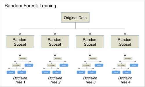
Random Forest
In order to understand the Random Forest, we first need to look at a slightly simpler model called a Decision Tree.
Decision Trees are probably familiar to many people in other contexts, and most would likely recognise the general branching structure based upon different conditions. In supervised learning the underlying concept is the same, that is to try and construct a tree where the branches enable us to differentiate between different categories.
For example, suppose that we wish to differentiate between Oranges, Apples and Bananas. One very simple decision tree might look something like this:
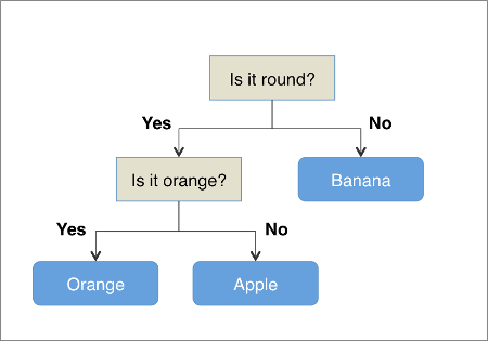
For certain types of problems, Decision Trees can be very powerful and they have the benefit of being fast to train and test. One issue, however, is that they tend to “overfit” the data. This means that the model they construct tends to be far too specific to the exact training data provided, and the model is not able to generalise very well when making predictions on new examples.
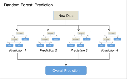
One way to combat this overfitting is to construct a large number of different Decision Trees and combine the output of all of the trees when making predictions. Each tree is 'grown' using a slightly different version of the training data, and the hope is that each tree will create a slightly different model and thus the algorithm can capture more of the nuances of the underlying problem and better generalise to new data.
This combination of decision trees is called a Random Forest and is an example of what is know as an 'ensemble' method. Random Forests are a very powerful classifier and find applications in many domains.
Support Vector Machine
The final model we will briefly explore is the Support Vector Machine.
Very informally, a Support Vector Machine attempts to build a model by finding a line (or lines) that separates the different categories in such a way that the data points are divided by a gap that is as large as possible. Once this line has been identified, prediction is simply a matter of identifying on which side of the line a new data point falls.
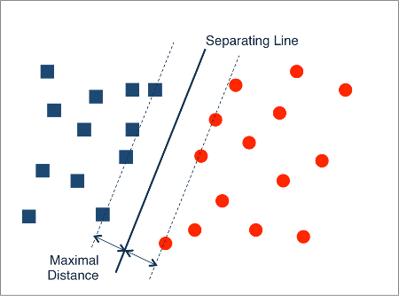
For a slightly more technical explanation we turn to linear algebra (feel free to skip the next few paragraphs). Suppose we are given training data whereby each example is represented by p different values; in this case we can consider our training data to be points in p-dimensional space.
The Support Vector Machine attempts to find a p-1 dimensional hyperplane (basically a generalisation of a straight line to p-1-dimensions) that separates and also maximises the gap between the categories.
The model described so far is called a Linear Support Vector Machine. One common problem with this approach is that is often not possible to find a separating straight-line or plane given only the existing data points.
Consider the following example in one dimension:
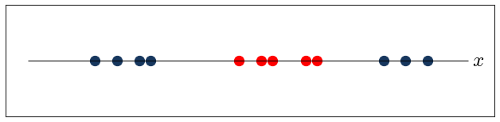
Here it is impossible to find a single straight line that separates the red and blue points.
Look at what happens, however, when we project the data into two dimensions, say by plotting $ x^{2} $ against $ x $.
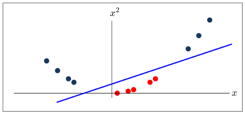
In this higher-dimensional space it is now possible to find a straight-line that separates the two classes.
This is an example of non-linear classification using Suport Vector Machines. Some common transformations to higher dimensions are Polynomial (such as the example above where the data is transformed to some power of itself), as well as using what is called the RBF kernel.
In practice these transformations are calculated using what is called the "kernel trick".
Algorithm Optimisation
Before moving on we must say something about the need for optimisation in supervised learning. For each of the models mentioned above, there are specific choices that must be made at the start when when the model is initialised prior to training.
For example for the k-Nearest Neighbours algorithm we must decide on the value of k and the definition of ‘closeness’. For Random Forests, among other things, we need to specify the number of decision trees to have in the forest. Similarly, for Support Vector Machines, there are a number of parameters that need to be specified.
These parameters are called hyper-parameters, and in general different choices for the parameters can result in different outcomes for the model in terms of predictive performance. For instance, a kNN algorithm may make very different predictions based upon whether it is looking at the nearest 3 vs. 10 neighbours.
Thus one key task when ‘training’ a machine-learning algorithm is to identify the values for the hyper-parameters which give the best results for the problem under consideration. This is called hyper-parameter tuning, and one of the most common approaches is called a grid-search.
In a grid-search we specify up-front a range of values for each hyper-parameter, and then train and test a model using every possible combination of these parameters. The values that give the best result during training (importantly not using the ring-fenced testing data), are then said to be the optimal parameters.
5. Traditional Machine Learning: Features
We have now looked at some examples of common machine learning algorithms that can be used in classification problems. However, for each of these algorithms, we must also decide on the nature of the data to use during training in the hope of creating the best predictive model.
Ultimately what we are looking for is the best possible representation of each of the different data points (in this case images), subject to a number of considerations, including:
- The representation must have sufficient information to be able to group together examples from the same category, but also to differentiate between different categories.
- At the same time, we want to avoid as much as possible the overfitting problem we mentioned earlier, that is we don’t want to provide so much detail that the model is not able to generalise well when used on new data.
Such representations of the data that are typically called features.
For the problem of image classification we need to begin by understanding the way images are represented digitally. Although we see images visually, a computer just sees them as a series of numbers. To illustrate this, look at the following picture consisting of a grid of 16 x 16 squares :
![]()
Each square represents one pixel in the image. We can think of a pixel as being the basic building block of images, where each pixel has a particular shade of grey associated with it. By laying out pixels of different shades next to each other it is possible to create more complex patterns and shapes.
Furthermore, we can specify the particular shade of grey of a given pixel using a single number and so the image above can be represented using a matrix of 16 x 16 = 256 numbers.
Now let us look at a similar image but in colour:
![]()
Here the principle is the same, with each pixel having a specific colour, however in this case we need three numbers rather than just one in order to specify the colour. These three numbers specify the shades of Red, Green and Blue which are combined to produce any desired colour. (Note: there are alternative representations of colour, however this RGB representation is one of the most common).
For example, the pixels with this colour:
![]()
can be specified by (Red = 0, Green = 128, Blue = 0), while these pixels:
![]()
can be specified by (Red = 242, Green = 128, Blue = 88).
Thus the colour image can be represented by a matrix of 16 x 16 x 3 = 768 separate numbers, and this is how a computer 'sees' images.
For machine learning, one approach could be to use these Red, Green and Blue pixel colour values as the features, however you might imagine that this is not necessarily the best approach:
- The number of individual features can become very large very quickly; for example our images have 512 x 512 pixels, meaning each individual image requires 786,432 different numbers to represent them
- Very large feature vectors can lead to problems of overfitting and,
- There is no reason to assume that the pixel-based representation will be the best possible representation
In my project I used a number of different approaches for extracting features from the images, and tested how well these feature combinations worked when used in conjunction with different algorithms. The main types of features I looked at are described in more detail below.
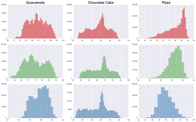
RGB Histograms
One of the simplest types of features that can be used are histograms of the Red, Green and Blue pixel values in the images, that is the relative frequencies of different colour intensities. It is not unreasonable to think that these differences might enable the classifier to distinguish between the food categories.
In fact, if we look at such histograms for three food categories, it is apparent that the colour distributions are quite different:
Edges
Another fairly simple and common type of feature are so-called Edges. An edge is defined by a discontinuity between pixels, which is basically an area where there is sufficient difference between pixels of one colour and another that an edge appears in the image.

Image by JonMcLoone at English Wikipedia, CC BY-SA 3.0, https://commons.wikimedia.org/w/index.php?curid=44894482
Typically you would count the number of edges within a given image or sub-region of an image, although in the field of computer vision there are other ways of using edges, for example looking at their orientation too (i.e., how many are vertical vs. horizontal etc.)
Corners
In addition to edges, one can also look at the number of corners within an image or image-region, where a corner is defined as the meeting point of two edges.
Meta-Approaches
It is important to note that features are typically not used in isolation but are combined together to try and come up with richer representations of the underlying examples.
For example we might use a set of features that is a combination of RGB Histogram values, plus the number of edges, plus the number of corners.
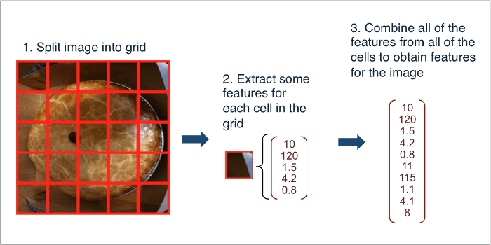
Another way one can combine features for a given image is by splitting the image into sub-regions, extracting features for each of the sub-regions, and then aggregating them all together into a complete representation of the overall image.
6. Deep Learning & Neural Networks
The general machine learning techniques discussed so far form the basis of what was the standard approach to computer vision for a long time. However in the past few years these techniques have been replaced by new approaches based on Deep Learning, and in particular models called Convolutional Neural Networks.
Convolutional Neural Networks, or CNNs for short, are currently considered to be "state of the art" in computer vision, and have also achieved success in many other areas and applications. In fact, in some very specific problems, CNNs are able to achieve greater accuracy than humans.
I will give a very brief introduction to Convolutional Neural Networks in order to motivate this approach.
Neurons
Let us start with the idea of a 'neuron', which is fundamentally nothing more than a very simple function that takes an input and produces an output dependent on two parameters that are intrinsic to that neuron, called its weight and bias:

Thus, in the example above, if X is 3, w is 1.2 and b is -6, the neuron would return an output of $ 3 \times 1.2 - 6 = -2.4 $.
This particular neuron is not that interesting as all it gives us is a simple linear function. We therefore introduce the concept of 'Activation', which is a way of ensuring that neurons do not produce output all of the time, only some of the time based on certain conditions:
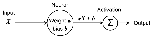
In the diagram above:
- The neuron receives input X
- The linear transform wX + b is calculated
- The result is passed through an activation function, ∑
- The final output depends on the nature of the activation function.
Probably the simplest choice for the activation function is what is called the Step function:
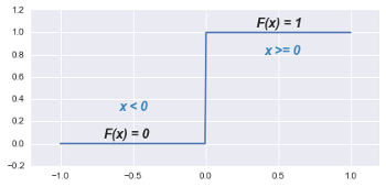
If the Step function receives a negative input (x < 0), then it returns an output of 0, while for inputs greater than or equal to 0, it returns an output of 1.
In practice this function does not behave in a mathematically nice way so typically the activation functions used will look more like these:
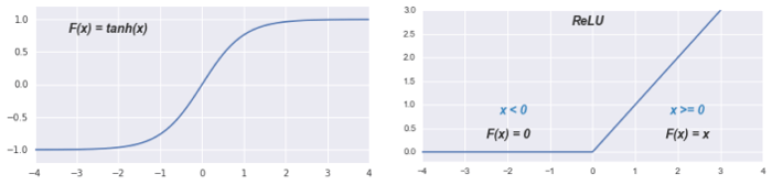
This concept of activation is where the name 'neuron' comes from, as these functions behave similar to biological neurons that 'fire' or 'don't fire' depending on the inputs they receive.
Networks
A single neuron on its own cannot do very much, however we can build up more and more complexity by combining many of these neurons into layers, and then connecting the layers together, for example as in the diagram below:

Image by Glosser.ca - Own work, Derivative of File:Artificial neural network.svg, CC BY-SA 3.0, https://commons.wikimedia.org/w/index.php?curid=24913461
Ultimately this is just a pictorial representation of a complicated function that:
- Receives an input or inputs
- "Propagates" the input through each neuron in each layer of the network, during which the output of one layer becomes the input to the next layer
- At each neuron applies the simple function above using the relevant weight, bias and activation
- Returns an output which is dependent on the value of all of the different parameters of all of the neurons in the network
In fact it can be shown that, with appropriate choices for each of the parameters, this sort of model can approximate any arbitrary function (as long as it is mathematically 'nice'), which means that it has the potential to be very powerful.
In the specific example above, there is one 'hidden' layer which sits between the input and output layers. Networks which have many hidden layers are called deep networks, and for this reason we talk about Deep Learning.
Training a Network
Once again we return to the idea of training a model using a set of inputs in conjunction with desired output. In this case the model is a network of connected neurons, and training involves adjusting the parameters of each neuron in order to maximize the total number of correct predictions emerging from the network.
Although the model looks very complex, the key ideas behind the training procedure turn out to be relatively simple. There is just one missing ingredient we need which is some sort of cost or loss function to measure how wrong the network outputs, or predictions, are.
When the predictions are very different from what they should be, the loss should be high, and as the predictions get closer to reality, then the loss should decrease toward 0. We can use this loss function during training to understand how to tweak the parameters in order to lead to better predictions.
To understand the training procedure let us look at a very simple toy example for a single neuron with only weight and no bias. During training, the procedure is:
- Start with a fixed input, X
- Pass X through the neuron, and calculate its output wX
- Compare the output to the desired result (in this case 1.00) and calculate the loss associated with the current output
- Slightly modify the neuron parameter w in such a way as to decrease the loss on the next pass
- Repeat until there do not seem to be any improvements.
This procedure is demonstrated in the animation below. Click on the button to start the training procedure and watch how the weight parameter, output and associated loss evolve.
For the mathematically inclined, this problem is nothing more than standard optimisation where we have a function F that takes an input x and, by using parameters W and B, returns an output C.
We wish to find the values of W and B that minimize C for a given input x.
We can use calculus to find the gradient of this function at x, and when we tweak the parameters, we do it in the direction of decreasing gradient of the function.
Although we have only illustrated training for a single neuron, ultimately the same basic procedure can be used to train very large and complex networks by taking advantage of two key ideas.
The first is a technique called backpropagation which enables us to calculate the gradient for many different types of networks and neurons connected together in different ways.
The second is the use of very efficient computer-based implementations of linear algebra and in particular vector and matrix multiplication, which lets us quickly perform the relevant calculations on very large inputs, or even to process multiple inputs at the same time.
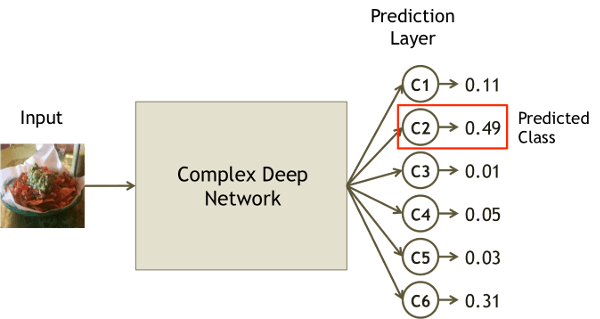
Predictions
In any network, the last layer typically corresponds to the categories that are being used for classification, where each neuron corresponds to a particular category. Then, when we make a prediction, it is based upon the neuron in the last layer with the highest activation, or output.
Convolutions
Although neural networks like the ones mentioned above are powerful, it turns out that for problems like computer vision even better results can be obtained by using a number of innovations. Thus far we have only looked at neurons that are "fully connected", that is in each layer (except the input and output layers) every neuron is connected to every other neuron in the preceding and following layers.
One key challenge associated with fully-connected networks, especially when using very high-dimensional data such as images, is that the number of required parameters can become too large to feasibly carry out the required computations, especially when using readily-available hardware.
For example, if we were to use 256 x 256 colour images as inputs, and supposing the first hidden layer has 1000 neurons, then just the initial weights to the input layer would require nearly 200 million parameters.
Furthermore, this "fully-connected" model is not always sufficient to capture all of the underlying complexities and nuances of the data, such as complex patterns that can appear in many different locations in an image.
However, by strategically combining other types of layers with different underlying connections, it is possible to achieve greater prediction accuracy while using fewer overall parameters.
One of the key types of layers used in state-of-the-art models is called a convolution layer.

Image by Aphex34 - Own work, CC BY-SA 4.0, https://commons.wikimedia.org/w/index.php?curid=45659236
Unlike a fully connected layer, a convolution layer does not "look" at the whole image in one go, but instead can be thought of as scanning across the image one piece at a time. During training the parameters of the convolution layer are modified as it attempts to detect underlying patterns that can be used for identifying different types of images.
These convolution layers can be stacked up, one after the other, and it turns out that earlier layers are typically used to identify very basic patterns, while later layers become tuned to identify more complex shapes made up of these simpler patterns.
This innovative architecture is also far more efficient in terms of parameters and calculations: single convolution layers used in practice can have only tens of thousands of parameters, and the best neural network used in this project has a total of approximately 60 million parameters.
While this is still a large number, it is far smaller than what could be required for a deep network consisting only of fully-connected layers.
Deep Learning in Practice
This basic introduction to Neural Networks and Deep Learning is not intended as a rigorous explanation, but more to give a brief overview of the core ideas behind this approach.
Before moving on to the results, it is worth noting two practical aspects of Deep Learning with CNNs:
1. Image Features
When using traditional machine learning models, we have to choose which types of features to feed into the model. Although in many cases the features are obtained using algorithms or other types of machine learning models, ultimately we are making a conscious decision in selecting the features ourselves.
In the case of CNNs, we simply feed in the raw images and then let the network itself identify and extract the key features. Not only is this less labour-intensive for the user, but the generated features tend to be superior and more useful.
2. Resources
CNNs can get very complex very quickly. Every single neuron has two parameters to optimize, its weight and bias, and CNNs typically have many thousands of neurons resulting in hundreds of thousands or even millions of parameters to be optimised during training.
As a result, training a CNN from scratch can take a long time and require a lot of training data. For example, for competition-winning CNNs, training is performed on more than a million images and is said to take three weeks or more.
All is not lost though, as there are techniques whereby we can take advantage of other people’s hard work, and instead of starting from scratch, work with networks that have been pre-trained on some other dataset.
Transfer Learning
There are two main approaches when it comes to working with pre-trained networks.
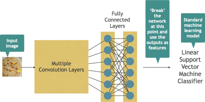
The first, Feature Extraction, is based on using the network to generate some features which can then be used to train a standard machine learning algorithm. Here we take advantage of the fact that CNNs are remarkably good at detecting the important features on their own and so we can save ourselves the trouble of trying to figure out the right sorts of features to use.
In this case all that needs to be done is to feed the training images into the network and then use the output from an intermediate layer as features for training one of the algorithms we have previously mentioned, say a Support Vector Machine or a Random Forest.
An alternative approach is called parameter Fine-tuning. Here we rely on the fact that the parameters of the network will already have been painstakingly optimised over many weeks, and so should already be pretty good at detecting image-based features.
As was previously mentioned, the initial layers of a CNN become tuned to detect very basic features, patterns and colours that are likely to exist in many different types of images. So rather than trying to train a network from scratch, we can start with a model that is already successful at classification in one domain, and simply spend some time tweaking the parameters very slightly in order to better adapt the network to our specific problem.
7. Results
In looking at the results, we will visualize performance in a couple of different ways:
- The overall accuracy of each model
- The performance on each food category
- The categories for which the models had most trouble
Overall Results
The chart below shows the overall classifier accuracy (more specifically the F1 score) for each of the different models that were tested. The results are plotted in order of performance from worst to best. You can move your mouse over each bar to see more details about the specific Algorithm, Data Features and Score for each attempt.
Looking at the chart, two things are clear.
First of all, progress using traditional machine learning approaches (models + pre-selected features) was slow and painful. Although the results did gradually improve, it took quite a long time to achieve an accuracy of 0.30 or above.
Secondly, the superiority of Deep Learning with CNNs is clear: all of the deep learning models (orange bars) performed better than traditional machine learning, and accuracy jumped significantly once we switched to deep learning approaches.
Per Class Results
Here we look at the evolution of the F1 score for each different food category. In this case, the results are plotted in the order they were obtained, that is attempt 1, followed by attempt 2, attempt 3 etc. Each line represents a different food category, and you can move the mouse over each line to see the relevant class and its final F1 score.
[Note that this chart has 46 different values on the $ x $-axis compared to 54 in the previous chart. This is because I did not obtain full per-class results for all of the initial training attempts.]
The first observation is that there is quite a wide variation in performance between categories, even when using the more powerful CNN-based models. For example, for the best classifier, the range of scores was as low as 0.61 for Steak, and as high as 0.91 for Guacamole.
From looking at this chart we can also say something about the overall process, notably that progress was not linear. At each attempt, both for traditional machine learning as well as CNNs, I tested different methodologies in the hope of improving on past results. In some cases this worked out, but in other cases these new combinations ended up giving worse scores than previous attempts.
Confusion Matrix
Now we turn our attention to the Confusion Matrix. Here we show the predictions for each different category, where the rows represent the true class, and the columns represent the predicted class. For example, the top left hand cell corresponds to pictures of Pork Chop correctly classified, and the next cell along on the same row corresponds to pictures of Pork Chop classified as being Lasagna etc.
The cell colour is indicative of the proportion of predictions that fall into that cell, with darker shading corresponding to a higher proportion. A perfect classifier would, for each category, place 100% of the predictions for that class into the cells on the diagonal line that goes from the top-left to bottom-right corners.
Thus, what we are looking for in the confusion matrix is for the cells on this diagonal line to be shaded very dark blue, with all other cells being shaded very light grey.
The initial starting point for the matrix is the results of a purely random model, that is to say a model where each prediction is based upon drawing food categories out of a hat. To explore the confusion matrix for different attempts you can either use the slider at the top, or press the Run Simulation button to cycle through the results of each of the different models. You can also hover over individual cells to see the exact proportions of predictions.
If we look at the confusion matrix for the best performing model, overall the picture looks very good, with a good amount of dark shading on the diagonal, and generally lighter cells everywhere else. However there are a couple of outliers that stand out:
- 18% of Steak images are classified as being Pork Chop
- 10% of Pork Chop pictures are classified as being Steak
What we are seeing is that the model has a particularly hard time distinguishing between these two categories, perhaps understandably as a cooked pork chop can look quite similar to a cooked piece of steak, particularly in a low-quality image.
Class Predictions
We saw above how different food categories can be "confused" for each other by the classifier. In this final chart we look more closely at how this confusion changes for each particular category using the different models.
The chart shows, for a given food category, what % of the test images are predicted as belonging to each class. The bar for the true category is shown in blue, and all incorrect categories are shown in green.
For example, the initial picture shows that for Pork Chops, just under 10% are correctly classified, and in general the predictions are distributed fairly evenly across all categories.
For each class you can see how its predictions are distributed as the classifiers evolve either by dragging the slider to a particular attempt, or by pressing the Run All button. Once again the order of the models is based upon the order that they were created and tested.
In general, for any given category, what we see is that early on the predictions are all over the place with the true class sometimes dominating and sometimes not, and then we we reach the CNN-based models around attempt number 40, all of a sudden the true class dominates the model's predictions.
8. Visualizing a Convolutional Neural Network
One benefit of many of the 'simpler' machine learning algorithms is that it is easier to visualize conceptually how they are working 'under the hood'.
For example, a k-Nearest Neighbours classifier is simply finding the 'closest' data points and making a prediction based upon the categories of these neighbours.
The maths behind a Support Vector Machine is more complicated, however we can at least imagine a series of straight lines separating different data points of different classes.
Random Forests can seem more like a black box, but we can still try and picture a large number of different decision trees, each taking slightly different features into account, and then combining predictions from each one into an overall prediction.
[Note that this refers to conceptual rather than practical visualization. In reality most non-trivial examples will consist of high-dimensional data which is much harder to visualize.]
Convolutional Neural Networks however are so complex, with many different types of neurons stacked into tens or even hundreds of layers, that is is much harder to come up with a simple explanation for how they are working. Having said that, there are a few tricks for visualizing what these networks are doing which can start to shed some light on the underlying model.
Convolutions and Patterns
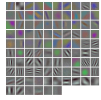
We saw earlier how one of the key elements behind the CNN is the convolution layer, which can be thought of as scanning across the image, looking for particular patterns in each part of the picture. One of the first things we can visualize is what some of these patterns might look like. This makes the most sense for the very first convolution layer which is applied directly to the raw image.
Here we can see very basic patterns such as straight edges of different orientations as well as simple blobs of different colours.
High Activation Images
An alternative approach to visualizing what is happening in each layer is by looking at images that maximally activate a given neuron.
Recall the concept of activation which was introduced for individual neurons whereby, depending on the input, the neuron's output can very from being very low to very high. This means that when a particular neuron is activated in the network, there must be some combination of pixels in the input image which is causing this activation.
What we can do is to try and artificially create a combination of pixels which results in the highest possible activation for this neuron, thus getting a sense of what sort of patterns, shapes or colours are causing different neurons to 'fire'.
Mathematically we take advantage of the fact that we already have a well-behaved function that was optimised to find the set of parameters resulting in the best overall predictions. We now take a similar optimisation approach, however this time rather than leaving the image fixed and varying the weights, we instead leave the weights fixed and vary the image pixel values in order to maximize the activation, or output, of a given neuron.
For example, here are synthetically generated images for two neurons in the prediction layer:
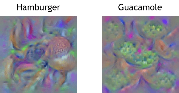
Although this does not produce pictures that look exactly like Hamburgers or Guacamole, it is certainly possible to discern recognizable structure, texture and colour in these images.
We can do the same for the different convolution layers in the network which, you will remember, are theoretically detecting different patterns at varying scales.
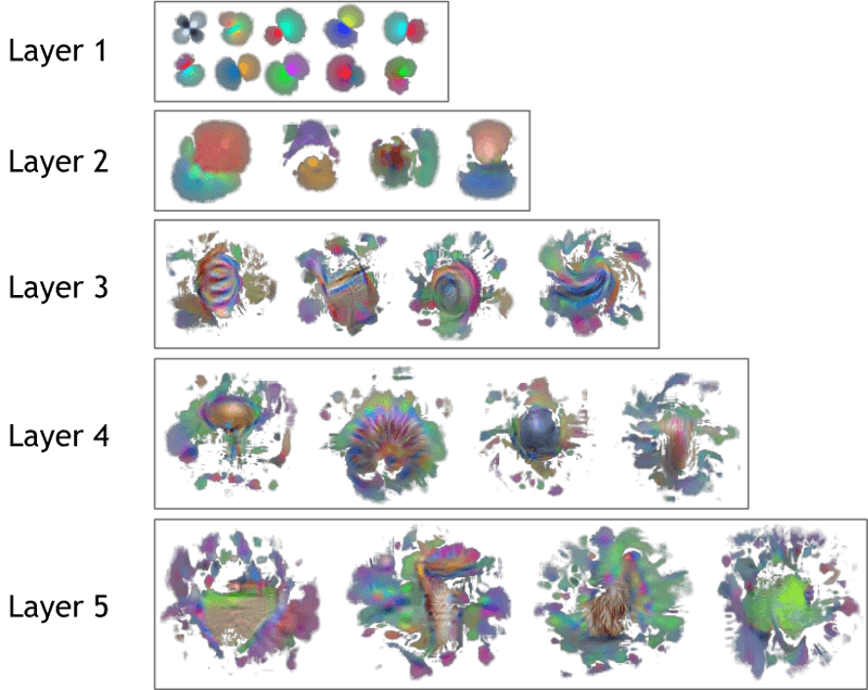
Here we can see two things quite clearly. First, as expected, the initial layers are activated by simple patterns, whereas later layers look for more complexity. Secondly, the field of vision of each layer increases as we go deeper into the network. For example the first layer looks at very small sub-regions of the image, whereas by the last layer, the convolution 'filters' are receiving input from a much larger area.
In reality most of the food items being classified do not have very distinctive shapes or colours, and so it is quite hard to interpret some of these patterns being detected by the different layers. These visualizations become a lot clearer if we look at similar synthetic images for the original network prior to fine-tuning on our food dataset.
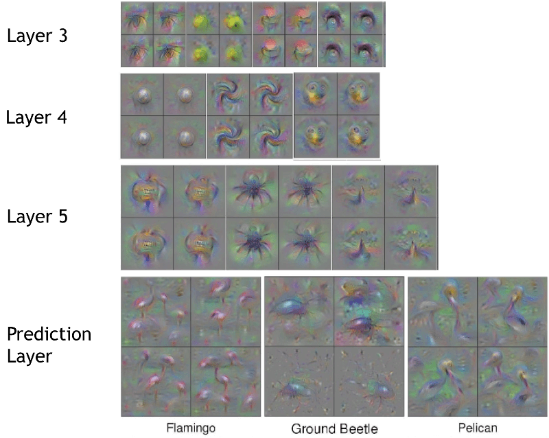
Source: Understanding Neural Networks Through Deep Visualization
9. Summary
Overall this was a fantastic learning experience that gave me the opportunity to work with both traditional machine learning as well as deep learning models. Working on a tangible, and at times messy, problem has definitely been the best way for learning about how some of these models are applied in the real world and the associated challenges.
In terms of computer vision, it is clear why Convolutional Neural Networks are the current state-of-the-art approach given the relative ease of obtaining good results in a relatively short space of time.
There is still a lot of work that could be done to achieve even better results for classifying food pictures, including:
- Expanding the approach to use all 101 food categories from the dataset
- Fine-tuning a more recent network that has achieved better results (i.e., GoogleNet, ResNet etc.)
- Investing more time in optimising parameters during fine-tuning
- Training multiple models and aggregating the predictions (an ensemble approach)
- Expanding the methods to include object detection for identifying multiple food types in one image.
References
The code for the final CNN-based model along with a full report and presentation can be found on GitHub.
An excellent introduction to Convolutional Neural Networks for Computer Vision is the Stanford CS231n course.
The network visualizations were created using the Deep Visualization Toolbox.