Making a Streetmap in Matplotlib
There are a lot of options nowadays for making maps programmatically (especially in Javascript) such as Leaflet and CartoDB.
However, there may be times where you want to include a map in a Jupyter notebook, or just create something yourself from scratch.
A solid, fairly easy-to-use option for Python is Matplotlib's Basemap extension.
Below is an example demonstrating how to use Basemap to create a streetmap of Mexico City, overlaid with neighborhood names.
Getting Setup
To add detail to the map, it will be good to have shapefiles for roads as well as neighborhood (colonia) boundaries and names.
Openstreetmap data for roads can be downloaded from: http://download.geofabrik.de/osm/north-america/mexico-latest-free.shp.zip
Once you extract the zip file, inside the folder you will find the following files:
- gis.osm_roads_free_1.cpg
- gis.osm_roads_free_1.dbf
- gis.osm_roads_free_1.prj
- gis.osm_roads_free_1.shp
- gis.osm_roads_free_1.shx
The neighborhood data comes from http://shapesdemexico.wixsite.com/shapes/agebs. Similarly, inside the folder are various files with extensions .dbf, .shf etc.
In both cases, the files we are interested in are those with a .shp extension.
If we want to filter these or integrate them with other data, we can load them into a PostgreSQL database and perform whatever analyses we want there.
Create a database:
createdb mapping
Add the PostGIS extension:
psql mapping -c 'CREATE EXTENSION postgis'
Load the street and neighborhood data:
shp2pgsql -s 4326 gis.osm_roads_free_1.shp roads | psql mapping
shp2pgsql -s 4326 Colonias.shp colonias | psql mapping
These last two commands will load the roads and colonias shapefiles into tables called roads and colonias respectively in the mapping database.
Once you have performed any analyses you need, you can re-extract relevant shapefiles using the psql2shp command.
For example, we'll extract Primary and Secondary roads, Motorways and Residential streets that fall within a box bounded by latitude / longitude coordinates for central Mexico City:
pgsql2shp -f extracted_roads -h localhost -u USERNAME mapping
"SELECT osm_id, geom FROM roads
WHERE fclass IN ('primary', 'secondary', 'motorway', 'residential')
AND ST_Within(geom,
ST_SetSRID(ST_GeomFromText('POLYGON((-99.22 19.33, -99.22 19.45,
-99.12 19.45, -99.12 19.33, -99.22 19.33))'), 4326));"
Similarly, extract the Colonias along with their names within the same bounding box:
pgsql2shp -f extracted_colonias -h localhost -u USERNAME mapping
"SELECT objectid, sett_name, ST_Force2D(geom) FROM colonias
WHERE ST_Within(geom,
ST_SetSRID(ST_GeomFromText('POLYGON((-99.22 19.33, -99.22 19.45,
-99.12 19.45, -99.12 19.33, -99.22 19.33))'), 4326));"
Creating the map
In order to actually draw the map, we'll need pyplot (as normal) as well as the Basemap extension:
%matplotlib inline
import matplotlib.pyplot as plt
from mpl_toolkits.basemap import Basemap
import numpy as np
Start by initializing a blank map:
fig, ax = plt.subplots(figsize=(10,15))

m = Basemap(
    resolution = 'c',
    projection = 'merc',
    llcrnrlon=-99.22, llcrnrlat= 19.33, urcrnrlon=-99.12, urcrnrlat=19.45)

m.fillcontinents(color='#f0f0f0')
The key arguments when initializing the map are:
resolution='c'
This sets the resolution to use for plotting boundaries, for example country borders. In our case we are zoomed-in to a specific city, so this does not really apply.
projection='merc'
The type of projection to use when drawing the map. For this map we are using the Mercator projection.
llcrnrlon=-99.22, llcrnrlat= 19.33, urcrnrlon=-99.12, urcrnrlat=19.45
The region to be mapped, specified by the latitude and longitude of the lower-left and upper-right corners. This can also be specified by coordinates for the center of the map along with the width and height of the map.
m.fillcontinents(color='#f0f0f0')
Finally, this sets the background color of continents (land) to be light grey.
All of this results in a blank canvas:

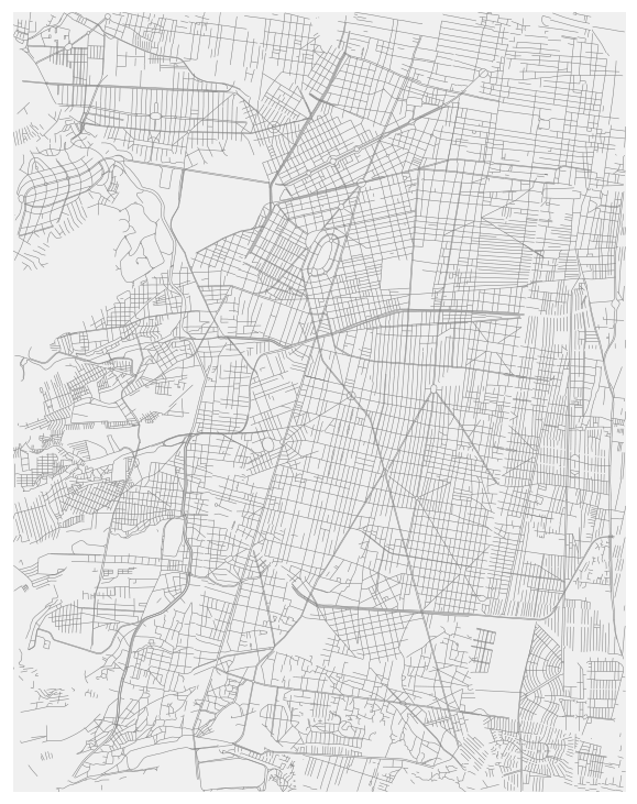
Adding the Roads
Noe we can go ahead and draw the roads and streets that we extracted earlier.
Using the same initialization code as above, we can simply add the lines:
m.readshapefile('extracted_roads', 'roads', drawbounds = True,
                color='grey')
This loads the .shp file created by the psql2shp command, and then
drawbounds = True, color='grey'
tells Basemap that we wish to draw the shapes included in the file on the map canvas using a grey line.
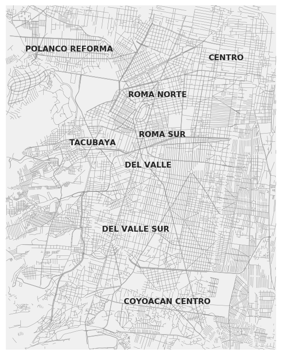
Adding Neighborhood Names
Before we can add the neighborhood names, we need to define a function for finding the center of a shape (defined by an array or coordinates):
def centeroidnp(arr):
    length = arr.shape[0]
    sum_x = np.sum(arr[:, 0])
    sum_y = np.sum(arr[:, 1])
    return sum_x/length, sum_y/length
Now we can add the colonias shapefile to the map:
m.readshapefile('extracted_colonias', 'colonias', drawbounds = False)
In this case we set drawbounds=False to specify that we don't want Basemap to add the shapes automatically.
If we were to plot all of the colonia names on the map, it will be too crowded, so let's just use a few specific names:
names_of_interest = ['DEL VALLE', 'POLANCO REFORMA', 'COYOACAN CENTRO',
                    'CENTRO', 'ROMA NORTE', 'ROMA SUR', 'TACUBAYA',
                    'DEL VALLE SUR']
Finally add these names to the map, plotting them in the center of their respective neighborhoods:
colonia_names = [c['SETT_NAME'] for c in m.colonias_info]

for name, shape in zip(colonia_names, m.colonias):
    if name in names_of_interest:
        x, y = centeroidnp(np.array(shape))
        ax.text(x, y, name, ha='center', va='center',
        fontsize=16, weight='bold', zorder=20, color='#252525')
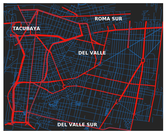
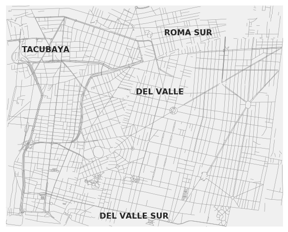
Zoom-In
We can zoom-in on a particular part of the city by adjusting the latitude and longitude of the bounding box:
m = Basemap(
    resolution = 'c',
    llcrnrlon=-99.195, llcrnrlat= 19.37, urcrnrlon=-99.145, urcrnrlat=19.41)
Let's include smaller roads, and this time we'll also extract the road type fclass:
pgsql2shp -f extracted_roads -h localhost -u simonbedford mapping
"SELECT osm_id, ST_MakeLine(geom), fclass FROM roads
WHERE ST_Within(geom,
ST_SetSRID(ST_GeomFromText('POLYGON((-99.195 19.37, -99.195 19.41,
-99.145 19.41, -99.145 19.37, -99.195 19.37))'), 4326));"
Change the Colors
Give the plot a dark background:
m.fillcontinents(color='#252525')
We'll also color the roads according to their type:
- A thick red line for primary & secondary roads and motorways
- A thin blue line for other roads
Define a custom function for obtaining the line color and width:
def line_styling(road_type):
    if road_type in ('primary', 'motorway', 'trunk', 'secondary'):
        return 3, '#F11810'
    else:
        return 1, '#2167AB'
Import the shapefile but don't automatically draw the roads:
m.readshapefile('extracted_roads', 'roads', drawbounds = False)
Instead, loop through each road and add it to the map with its format based on the type of road:
road_types = [r['FCLASS'] for r in m.roads_info]

for shape, road_type in zip(m.roads, road_types):
    lw, c = line_styling(road_type)
    x, y = zip(*shape)
    m.plot(x, y, marker=None, color=c, lw=lw)
Change the color of the neighborhood names from black to white:
ax.text(x, y, name, ha='center', va='center', fontsize=16,
        weight='bold', zorder=20, color='white')